Demo

Click or drag on the canvas to interact. Alignment, rotation, and grid controls are not currently supported.

Credits

The interactive demo adapts infrastructure from Self-Organizing Textures (Mordvintsev et al., 2021) on Distill, published under the MIT License. The GLSL shader is re-written.

NCA models were trained using the NCA node in SideFX Houdini. Training datasets were generated in Houdini Copernicus.

The Houdini NCA source code was authored by Jakob Ringler.

Intro

The NCA nodes introduced in Houdini 22.0 handles training and exports .onnx. Here I tried to export weights from .pt, and migrate the forward pass from .py to OpenCL (for Houdini COP) and GLSL (for the WebGL demo above), and HLSL (for Unreal Engine).

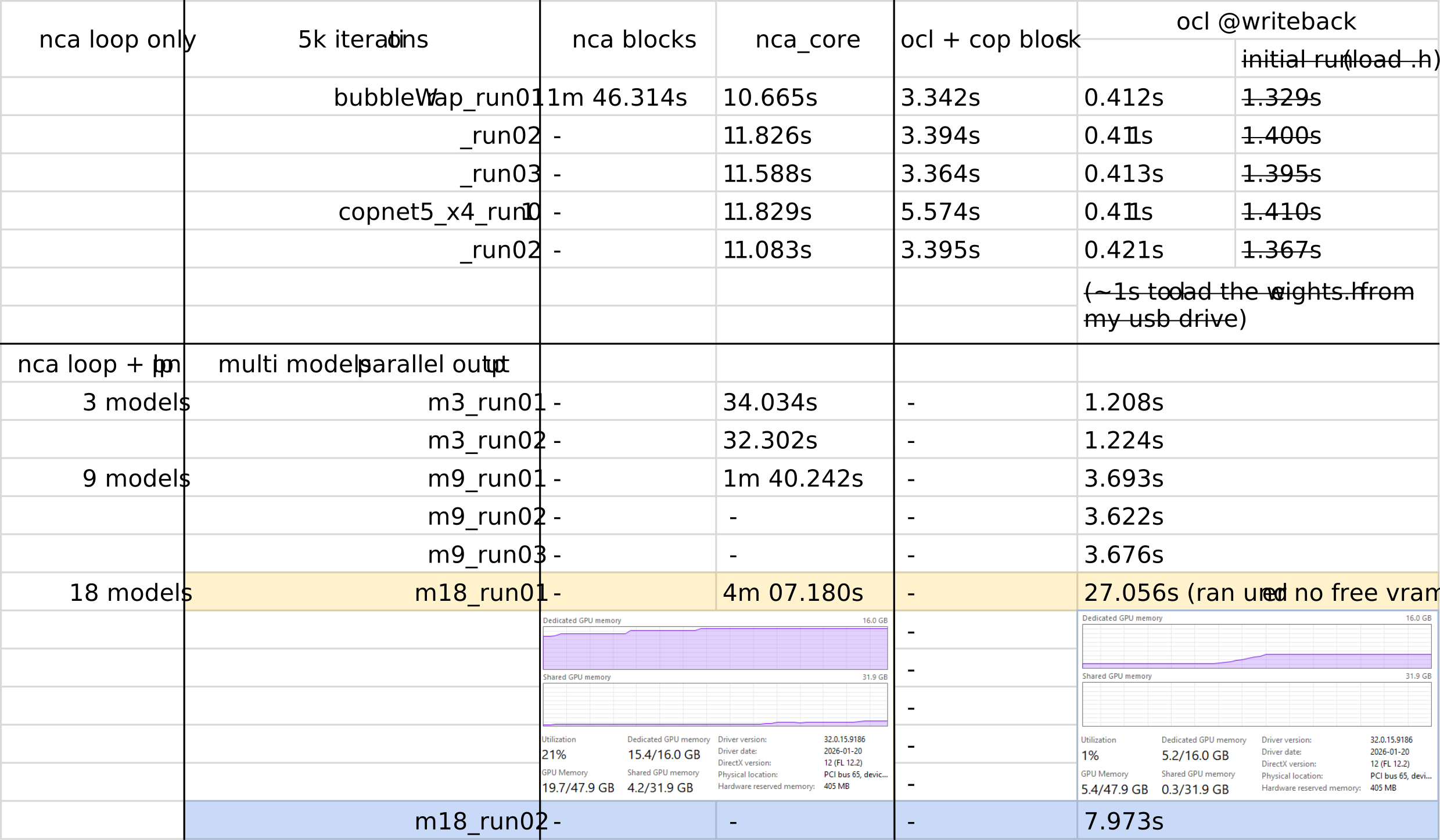
I benchmarked 5,000 NCA iterations across the original COP Block loop, Houdini’s nca_core, OpenCL with COP Blocks, and the final @WRITEBACK kernel. The lower half measures parallel NCA + LPPN output with 3, 9, and 18 models.
The results produced a clear improvement in both speed and VRAM usage:

What is NCA

Houdini’s Neural Cellular Automata system trains a neural network to learn local rules, then applies those rules back to a tileable pattern. The process has two parts: NCA Core evolves the pattern, and LPPN Decode turns that pattern into a detailed image.

NCA Core

The NCA Core runs the cellular simulation on a grid. Each cell stores a small hidden state, reads its 3x3 neighbourhood, and applies the same learned update rule over and over. Because every cell only reacts to nearby information, local changes spread across the grid and gradually organize the cells into larger shapes. The shared rule keeps this process consistent across the whole grid at every step.

Put simply, NCA Core repeatedly updates each cell from its neighbours so a small cellular state can grow into the image’s overall structure.

LPPN Decode

The NCA grid is an internal representation, so it still needs to be translated into visible pixels. LPPN Decode reads the state of the matching NCA cell together with the pixel’s local position inside that cell, then converts that information into RGB. This lets a relatively small NCA grid describe a sharper, higher-resolution image without forcing the core simulation to run at full output size.

In short: LPPN Decode maps each low-resolution cell to the RGB values of its corresponding high-resolution pixels.

The Migration

Weights Export

Training produces .pt checkpoint files — one for NCA, one for LPPN. I use export_weights.py to read and write them to flat C arrays into .h files for OpenCL, .json for WebGL, and .wsh for Unreal Engine. The corresponding kernels #import or #include these at the top and see the weights as compile-time constants.

nca.pt         →  weights_from_pt()        →  W1[128*64]  B1[128]     W2[16*128]   →  model.h
lppn.decode.pt →  decode_weights_from_pt() →  L0w..L3b    WIRE_OMEGA  WIRE_SIGMA   →  model.decode.h

NCA

The model defines two layers in nca.py:

w1      1×1 Conv2d: 64 input → 128 output         W1 [128, 64] + B1 [128]
w2      1×1 Conv2d: 128 input → 16 output         W2 [16, 128], no bias

The shapes after squeezing: W1 is [128, 64], B1 is [128], W2 is [16, 128]. export_weights.py pulls them out:

# weights_from_pt
data = torch.load(path, map_location="cpu")
sd = data["state_dict"]
return {
    "w1": sd["w1.weight"].squeeze().numpy().astype(np.float32),  # [128, 64]
    "b1": sd["w1.bias"].numpy().astype(np.float32),              # [128]
    "w2": sd["w2.weight"].squeeze().numpy().astype(np.float32),  # [16, 128]
}

Then kernels imports the resulting weight arrays and uses W1, B1, W2 directly.

LPPN

lppn.py builds the decoder as an nn.Sequential in wire mode (I only supported wire mode not siren yet). Even indices are Conv2d (have weights); odd are Wire2DActivation — no parameters, nothing saved.

lppn.0    L0    Conv2d(18→44)    →    L0w, L0b
lppn.1    —     Wire2DActivation →    no parameters
lppn.2    L1    Conv2d(22→44)    →    L1w, L1b
lppn.3    —     Wire2DActivation →    no parameters
lppn.4    L2    Conv2d(22→44)    →    L2w, L2b
lppn.5    —     Wire2DActivation →    no parameters
lppn.6    L3    Conv2d(22→3)     →    L3w, L3b

export_weights.py reads only the even ones, plus two scalars #define WIRE_OMEGA / #define WIRE_SIGMA from the architecture dict:

# decode_weights_from_pt
return {
    "L0w": sq("lppn.0.weight"),  # [44, 18]
    "L0b": sq("lppn.0.bias"),    # [44]
    "L1w": sq("lppn.2.weight"),  # [44, 22]
    "L1b": sq("lppn.2.bias"),
    "L2w": sq("lppn.4.weight"),
    "L2b": sq("lppn.4.bias"),
    "L3w": sq("lppn.6.weight"),  # [3, 22]
    "L3b": sq("lppn.6.bias"),    # [3]
    "wire_omega": float(arch["wire_omega"]),
    "s0":         float(arch["s_0"]),
}

Forward Pass: NCA

The NCA core is the part that evolves the hidden cellular state. Each iteration runs the same small rule everywhere on the grid: read a cell’s local neighbourhood, turn that into a learned update, then apply the update only to a random subset of cells.

current state[16]
  -> Perception: read each cell's 3x3 neighbourhood with fixed filters
  -> Network: run the 64 perception values through W1/ReLU/W2
  -> Stochastic update: apply the 16-channel delta to about half the cells
  -> next state[16]

Perception

Each cell needs to know what’s around it. nca.py applies four fixed 3x3 filters to each channel:

self.register_buffer('ident', torch.tensor([[0.0,0.0,0.0],
                                            [0.0,1.0,0.0],
                                            [0.0,0.0,0.0]]))
self.register_buffer('sobel_x', torch.tensor([[-1.0,0.0,1.0],
                                              [-2.0,0.0,2.0],
                                              [-1.0,0.0,1.0]]))
# Split Laplacian into x and y components
self.register_buffer('lap_x', torch.tensor([[0.5,0.0,0.5],
                                            [2.0,-6.0,2.0],
                                            [0.5,0.0,0.5]]))
# lap_y is transpose of lap_x
self.register_buffer('lap_y', torch.tensor([[0.5,2.0,0.5],
                                            [0.0,-6.0,0.0],
                                            [0.5,2.0,0.5]]))

In opencl, perchannel_conv is unfolded into an explicit 3x3 accumulation. Each of the 16 state channels is processed by the identity, Sobel X, Sobel Y, and Laplacian filters, packing the 4 x 16 responses into perc[64]. The filter weights become compile-time constants:

state[16 ch]
    │  4 filters * 16 ch, 3x3 neighborhood
    ├── identity  → perc[c*4+0]
    ├── sobel_x   → perc[c*4+1]
    ├── sobel_y   → perc[c*4+2]
    └── laplacian → perc[c*4+3]
                  = perc[64]

__constant float SOBEL_X[9] = {-1,0,1, -2,0,2, -1,0,1};
__constant float SOBEL_Y[9] = {-1,-2,-1, 0,0,0, 1,2,1};
__constant float LAP[9]     = { 1,2,1, 2,-12,2, 1,2,1};

float perc[64];
for (int i=0; i<64; i++) perc[i] = 0.0f;

for (int dy=-1; dy<=1; dy++)
for (int dx=-1; dx<=1; dx++) {
    int nx = ((gx + dx) % W + W) % W;
    int ny = ((gy + dy) % H + H) % H;
    // load neighbor n[16] from state layers at (nx, ny) ...
    int k  = (dy+1)*3 + (dx+1);
    float ki = (dx==0 && dy==0) ? 1.0f : 0.0f;
    for (int c=0; c<16; c++) {
        perc[c*4+0] += ki         * n[c];  // identity
        perc[c*4+1] += SOBEL_X[k] * n[c];
        perc[c*4+2] += SOBEL_Y[k] * n[c];
        perc[c*4+3] += LAP[k]     * n[c];
    }
}

Network

perc[64] goes through two layers — w1 expands to 128 with ReLU, w2 collapses to 16 with no bias.

perc[64]
    │  W1[128*64] + B1  →  fmax(., 0)
    ↓
h[128]
    │  W2[16*128]  (no bias)
    ↓
delta[16]

float h[128];
for (int hi=0; hi<128; hi++) {
    float sum = B1[hi];
    for (int i=0; i<64; i++) sum += W1[hi*64 + i] * perc[i];
    h[hi] = fmax(sum, 0.0f); // ReLU
}

float delta[16];
for (int c=0; c<16; c++) {
    float sum = 0.0f;
    for (int hi=0; hi<128; hi++) sum += W2[c*128 + hi] * h[hi];
    delta[c] = sum;
}

Stochastic Update

Not every cell applies its delta — about half skip each step. The randomness in nca.py uses a sin-based hash:

def simple_hash(self, x):
    x = torch.sin(x * 0.10873) * 43758.5453
    x = x - torch.floor(x)
    x = torch.sin(x * 12.9898 + 78.233) * 43758.5453
    return x - torch.floor(x)

# in forward():
uniform = self.random_uniform(current_seed + 2.71828182846, b, 1, h, w)
udpate_mask = (uniform + update_rate).floor() * update_map  # ~50% pass
x = x + y * udpate_mask

Ported to OpenCL:

float nca_hash(float x) {
    x = sin(x * 0.10873f) * 43758.5453f;
    x = x - floor(x);
    x = sin(x * 12.9898f + 78.233f) * 43758.5453f;
    return x - floor(x);
}

float combined = @seed + 2.71828182846f + (float)gx * 0.1031f + (float)gy * 0.0973f;
float rng = nca_hash(combined);
if (rng >= 0.5f)
    for (int c=0; c<16; c++) s[c] += delta[c];

forward pass: LPPN

lppn.ocl runs at output resolution — one thread per output pixel, not per NCA cell. Each thread finds its NCA cell, computes where it sits inside it, and decodes the cell state to RGB.

Coordinates

lppn.py computes local coordinates — where within the cell does this pixel land, normalized to [-1, 1]:

cell_w = output_w / nca_w
x = torch.arange(output_w, dtype=torch.float32) + 0.5
x_in_cell = (x % cell_w) - cell_w / 2
u = 2.0 * x_in_cell / cell_w   # [-1, 1]
# same for v

In OpenCL, per-pixel:

float cell = scale_f;
float pu = 2.0f * (fmod((float)gx + 0.5f, cell) - cell * 0.5f) / cell;
float pv = 2.0f * (fmod((float)gy + 0.5f, cell) - cell * 0.5f) / cell;
int sx = (int)((float)gx / scale_f);  // NCA cell coords
int sy = (int)((float)gy / scale_f);
// load state at (sx, sy) → 16 floats

Then inp[18] = [pu, pv, 16 state channels]. In lppn.py, this is torch.cat([pe_batch, h0, h1, h2, h3], dim=1).

• pe_batch: two local-coordinate channels (pu, pv) for each output pixel.
• h0, h1, h2, h3: four groups of four channels, together holding the 16 NCA state values.
• dim=1: concatenate along the channel dimension.

So:

2 coordinate channels + 4 x 4 state channels = 18 channels

In OpenCL:

inp[0]     = pu
inp[1]     = pv
inp[2..17] = 16 NCA state values

Wire2DActivation

The activation function between each Conv layer. lppn.py:

def forward(self, x):
    z1, z2 = torch.chunk(x, 2, dim=1)   # split in half
    gabor    = torch.sin(self.omega_0 * z1) * torch.exp(-(self.s_0 * z1)**2)
    gaussian = torch.exp(-(self.s_0 * z2)**2)
    return gabor * gaussian

Wire2DActivation splits the 44 Conv outputs into two 22-value halves and pairs them by index.
For each pair, z1 drives the sine oscillation, while Gaussian terms from both z1 and z2 damp its amplitude.

Multiplying the three terms produces one value, so 44 inputs become 22 activated features.

// Conv(18→44) + bias
for (int hi = 0; hi < 44; hi++) {
    float sum = L0b[hi];
    for (int i = 0; i < 18; i++) sum += L0w[hi*18 + i] * inp[i];
    tmp[hi] = sum;
}
// Wire2DActivation: z1=tmp[0..21], z2=tmp[22..43]
for (int i = 0; i < 22; i++) {
    float z1=tmp[i], z2=tmp[i+22];
    float a=WIRE_SIGMA*z1, b=WIRE_SIGMA*z2;
    h0[i] = sin(WIRE_OMEGA*z1) * exp(-a*a) * exp(-b*b);
}

Layer Stack

L0 is the input layer.

Then h_layers=2, the model inserts two repeated hidden layers, L1 and L2;
each layer produces 44 values, then Wire2DActivation combines the two 22-value halves into 22 outputs.

L3 is the final linear readout from those 22 features directly to RGB.

inp[18]  ← [pu, pv,  state×16]
    │  L0: Conv(18→44) + Wire2D → h0[22]
    │  L1: Conv(22→44) + Wire2D → h1[22]
    │  L2: Conv(22→44) + Wire2D → h2[22]
    │  L3: Conv(22→3)
    ↓
rgb[3]

in Houdini COP

┌ Block Begin
│	↓
↑ NCA OpenCL (#import nca.h -> W1, B1, W2)
│	↓		 (seed = @cop_iteration)
└ Block End
      ↓
LPPN OpenCL  (#import lppn.h -> L0w..L3b, WIRE_OMEGA, WIRE_SIGMA)

Writeback

OpenCL

The Begin/End COP Blocks method above was the first version of the feedback loop. Then that loop was moved into the OpenCL kernel itself with @WRITEBACK.

The NCA pass cannot write directly into state0–state3 while neighbouring cells are still reading them.
The kernel therefore separates the update into two phases. At the end of @KERNEL, each thread repacks its updated s[16] into four temporary float4 output layers:

@out0.set((float4)(s[ 0], s[ 1], s[ 2], s[ 3]));
@out1.set((float4)(s[ 4], s[ 5], s[ 6], s[ 7]));
@out2.set((float4)(s[ 8], s[ 9], s[10], s[11]));
@out3.set((float4)(s[12], s[13], s[14], s[15]));

After that kernel pass finishes, @WRITEBACK copies the temporary outputs into the persistent state layers:

@WRITEBACK
{
    @state0.set(@out0);
    @state1.set(@out1);
    @state2.set(@out2);
    @state3.set(@out3);
}

The writeback state becomes the input to the next internal OpenCL iteration:

old: Block Begin -> NCA OpenCL -> Block End -> repeat

new: state0..3
         -> @KERNEL
         -> out0..3
         -> @WRITEBACK
         -> state0..3 for the next internal iteration

WebGL

The WebGL version uses the same ping-pong update. Each step reads from src and writes the next state into dst;
after the draw finishes, one line swaps them so that the new state becomes the next step’s input:

[this.src,this.dst]=[this.dst,this.src];

Unreal Engine Niagara Grid2D

Unreal Niagara’s built-in Grid2D simulation follows the same pattern. A Simulation Stage reads the current cell values from one Grid2D buffer and writes the updated values into another.
At the end of the stage or iteration, Niagara makes that output buffer the input for the next pass.
(Haven’t check its source code, but its behavior matches the same ping-pong update pattern.)